
Ashley Jones
Assignment 3: Activity 1
Graphs in the xb plane
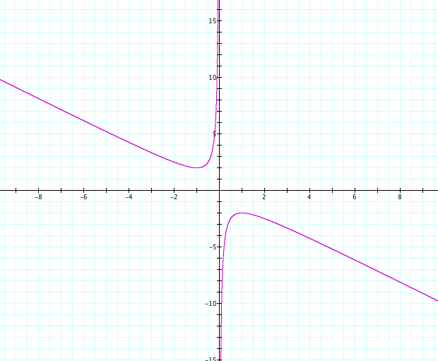
We are given the equation x^2 + bx + 1 = 0. To look further into this equation we can graph on the xb plane using Graphing Calculator. When we do this, we see the following graph:
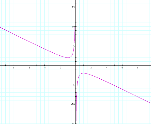
There are many ways that we can solve for the roots of this equation at any value of b. One way is to graph a horizontal line, such as b = 10, on top of the already existing graph of the equation. Below is an example of this where b = 6. We can see that in this example there are two negative real roots at b = 6, since the horizontal line crosses the graph of the equation twice in the second quadrant (where x is negative).
If we oscillate the value of b, for the horizontal line, between -10 and 10 we will be able to see in a more clear manner how the real roots of the equation x^2+bx+1=0 varies for each value of b. Below is an illustration of this as b varies between the values of -10 and 10.
By studying the above illustration, we begin to see the real roots of this particular equation as b varies. From the graph it is easy to see that when b > 2 the equation has two negative real roots, when b = 2 there is exactly one negative real root, when b < -2 there are two positive real roots (in the fourth quadrant), and when b = -2 there is exactly one positive real root.
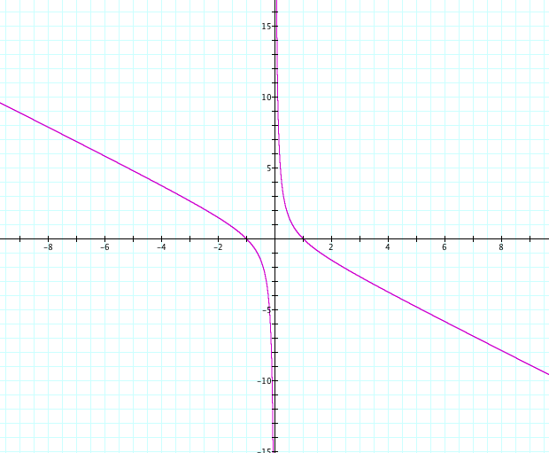
This illustration had me wondering, what would happen to the roots of the equation if we changed the value of c from +1 to -1? Therefore I started by graphing the original equation, but with c= -1. Below is the graph of x^2 + bx -1 =0 in the xb plane.
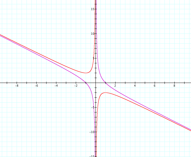
When looking at this new graph, I wondered how it related to the graph of the original equation where c = 1. Below I have graphed the original equation, as well as the second equation, where c= -1 to study how the two equations relate to one another. Looking at the graph, you can quickly see that the graph where c = -1 (purple) follows along the asymptotes of the original graph (red).
When finding the real roots of the equation x^2 + bx -1 = 0 we can see that there are always one positive real root and one negative real root no matter what the value of b is. This can be seen in the illustration below. On top of the equation where c = -1, I have placed a horizontal line where b varies between -10 and 10. As the horizontal line passes over the graph of the equation (purple) we notice that it is always intersecting at exactly one negative value of x and one positive value of x. We also notice that when b = 0, the two real roots are exactly x = -1 and x = 1.
Changing the value of c was very interesting, and altered the real roots of the equation dramatically. To look into this equation a little further on the xb plane, I created an illustration using the original equation but varying the value of c between -10 and 10. By doing this I was able to see what happens to the graph of the equation as the value of c varies. Below is the illustration of this exploration.
Studying this illustration we can see that when c is greater than 0 the equation will have either two negative real roots, one negative real root, two positive real roots, or one positive real root at any given value of b. We can also see that when c is less than 0 the equation will always have one positive and one negative real root for any value of b. If we take a look at the graph of the equation when c = 0 we find that the graph is of a linear function. Thus, we can determine that at any given value of b, the equation when c = 0 will have exactly one real root. An illustration of the equation when c = 0 can be seen below (purple). The horizontal line (red) again will show how the equation at c = 0 has exactly one real root at any given value of b.
This exploration is a great way to look at equations in other various planes. Also, it is a great way to explore the idea of real roots in relation to given equations. Many students might find this exploration helpful when trying to tackle roots of an equation.